The Big Picture

---

• How Are Economic Inequality & Growth Connected?
• 10 Thursday PM Reads
• How Much Slack Is in the Labor Market? That Depends on What You Mean by Slack
• Market Sell Off May Not Have Run Its Course Yet
• 10 Thursday AM Reads
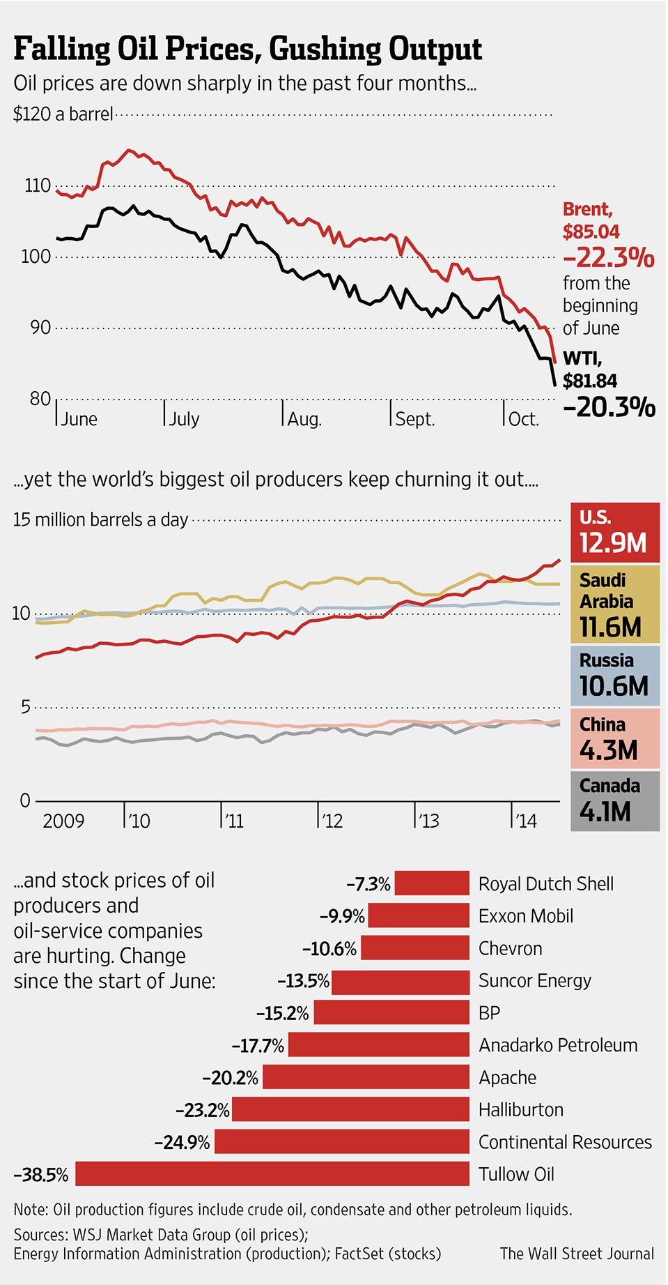
• Oil Glut Driving Prices Lower

How Are Economic Inequality & Growth Connected? Posted: 17 Oct 2014 02:00 AM PDT

10 Thursday PM Reads Posted: 16 Oct 2014 01:30 PM PDT My  afternoon train reads: • The Depressing Signals the Markets Are Sending About the Global Economy (The Upshot) • “Nine out of ten Forex clients lost money” (FT Alphaville) • Is the Global Financial Asset Portfolio the Perfect Indexing Strategy? (Pragmatic Capitalism) • OPEC Finding U.S. Shale Harder to Crack as Rout Deepens (Bloomberg) • Top 20 Financial Pundits To Follow On Twitter (Benzinga) • GOP voter ID law gets crushed: Why Judge Richard Posner's new opinion is so amazing (Salon) • Ready for a Patented Supreme Court Smackdown? (Bloomberg View) • Corporations used to pay almost 1/3 of federal taxes. Now it’s 1/10 (Vox) see also  Median Wealth Is Down by 20 Percent Since 1984 (CEPR) • Google Thinks Amazon Is Its Biggest Competitor. Here's Why. (Slate) • The Risks of Cheap Water (NY Times) What are you reading?     New Oil Bear Market? Source: Bespoke Investment Group

How Much Slack Is in the Labor Market? That Depends on What You Mean by Slack Posted: 16 Oct 2014 11:30 AM PDT How Much Slack Is in the Labor Market? That Depends on What You Mean by Slack Murat Tasci and Randal Verbrugge Federal Reserve Bank of Cleveland, 10.15.14           Estimates of labor market slack can diverge a great deal depending on how slack is defined. We calculate slack using five different concepts that all focus on a single labor market indicator, the unemployment rate. We show that the estimates all provide useful—but different—information. We argue that choosing the best measure of slack depends on the question being asked. If the question is, "Has the unemployment rate reached its new longer-run normal level?" then our answer is, "Almost." But significant uncertainty surrounds the estimates; and others may wish to consider additional labor market indicators. In the statement released after its July meeting, the Federal Open Market Committee (FOMC) noted a "significant underutilization of labor resources," which is to say that there is "slack" in the labor market. How much slack is open to debate. There are different ways to measure slack, and they don't always give the same answer. Indeed, some of these differences are reflected in the minutes of that same FOMC meeting: Participants generally agreed that … labor market conditions had moved noticeably closer to those viewed as normal in the longer run. Participants differed, however, in their assessments of the remaining degree of labor market slack and how to measure it. In this Commentary, we revisit the issue of labor market slack, focusing on a single labor market indicator, the unemployment rate. Using this single indicator, slack in the labor market means that the unemployment rate is above its longer-run normal level. But there are many different ways to measure this longer-run level and hence many different estimates of slack. We examine five different approaches to measuring the longer-run level of unemployment and provide some leading estimates of slack associated with each approach. We demonstrate that these different estimates have implied very different answers about the amount of slack in the labor market at various times. There is considerable uncertainty surrounding the estimates, so we cannot draw sharp conclusions about the amount of slack, or about differences between slack estimates. A forecasting exercise confirms that the various estimates provide useful—though different—information. We draw several conclusions. Like Rogerson (1997) and Svensson (2012), we conclude that different concepts of "long-run normal" are far from equivalent and are actually suited to different uses.1 Hence, "Is there significant slack in the labor market?" is a poorly-posed question, because "slack" has alternative definitions. If the question is "Has the unemployment rate reached its new longer-run normal level?" then—examining the estimates that derive from the appropriate concepts—our answer is: "Almost." Defining Slack To assess the current degree of slack, some economists argue that it is important to take account of a number of different variables simultaneously. However, in this Commentary, we take a narrow view and restrict attention to what is arguably the single most prominent measure of the state of the labor market, the unemployment rate. Using the unemployment rate as the labor market indicator, slack is defined as a current unemployment rate that is above the longer-run normal level of the rate. We denote this hypothetical normal level by un*t . Specifically, labor market slack equals the percentage point difference between the current unemployment rate and its normal level; in equation form, slack = unt – un*t. In this notation, un denotes the unemployment rate level, the asterisk denotes the fact that the long-run normal level is a hypothetical level, and the subscript t stands for "time period." We specify un* at a particular time because this hypothetical level might not be constant over time. For example, perhaps un*t was 6.5 percent in December 2012, but by July 2014 it had moved to 5.5 percent. Five Different Ways to Measure Normal Given that un*t is a hypothetical construct, there are a number of different methods for estimating it. We compare five and demonstrate that the choice of method can matter a lot. Estimates using each approach are plotted in figure 1. Trends in Job Flows One recent approach to measuring the longer-run normal level of the unemployment rate looks at trends in labor market flows. The modern theory of search unemployment recognizes that the unemployment rate depends on underlying labor market flows both into and out of unemployment. The idea is that the level of the unemployment rate is like the level of water in a pond: its level depends upon how fast water is rushing in and how fast water is rushing out. In the same way, the theory of search unemployment predicts that the long-run unemployment rate is a function of long-run trends in inflows and outflows. A prominent recent study using this approach is Tasci (2013). He estimates un*t with the underlying trends in these flow rates. Flexible Wage Counterfactual in a Sticky-Price Model A second recent approach involves creating a particular type of theoretical sticky-price model of the economy and then estimating it. In such models, wages and prices are "sticky," meaning that they cannot respond immediately to shocks. As a result, the unemployment rate in the models is often different from the hypothetical level un*t , the level that the unemployment rate would have been (under current conditions), had prices and wages instead been able to respond immediately to shocks. This level un*t can be considered the "long-run normal level" of the unemployment rate. In a prominent recent paper which conducts such analysis, Gali, Smets and Wouters (2012) call this un*t the "flexible wage counterfactual." In their model, labor market slack is part of the wage inflation Phillips curve, rather than the price inflation Phillips curve. Their estimate of un*t is quite volatile relative to the other un*t estimates we consider. Estimating Unobserved Components A third approach to measuring the longer-run normal level of the unemployment rate involves unobserved components modeling. The basic assumption in this approach is that an economic time series is composed of four unobserved parts: a trend part, a cyclical part, a seasonal part, and a random noise part. The economist observes only the sum of the four parts. Econometric techniques can be used to split the series into its four component parts and produce an estimate of each. When used in the context of the unemployment rate, the trend estimate at time t is sometimes used as the estimate of the long-run level un*t. A prominent recent example comes from Stella and Stock (2012). Forecasting A fourth approach to measuring the longer-run normal level of the unemployment rate involves forecasting. In this approach, a forecast of the long-run level of the unemployment is taken as the estimate of un*t. A notable recent forecasting model is presented in Beauchemin and Zaman (2011). Inflation A fifth approach to measuring the longer-run normal level of the unemployment rate is probably the oldest approach of the five we consider and relies upon the connection between inflation and labor market slack. The core idea here is that weak price or wage growth indicates the presence of slack in the labor market. If the idea seems unfamiliar, it may help to recognize that it is usually presented differently: inflation falls when unt is above un*t, and it rises when unt is below un*t. This relationship is a central part of the theory of the expectations-augmented Phillips curve, introduced in the late 1960s. The level un*t was originally termed the "natural rate of unemployment" and was taken to be the long-run normal level of the unemployment rate—and the only feasible target for monetary policy. In later theory, this un*t concept was termed the NAIRU (nonaccelerating inflation rate of unemployment). Here is the definition given by Joseph Stiglitz (1987): The NAIRU is … the rate of unemployment consistent with an unchanging inflation rate. When unemployment is below the NAIRU, there is pressure for the inflation rate to rise; contrarily, when unemployment is above the NAIRU, there is pressure for the inflation rate to fall. Stiglitz also argued that the NAIRU should instead be called the NIIRU (nonincreasing inflation rate of unemployment). This is because "accelerating" inflation is now almost certainly impossible in OECD countries, given the way that monetary policy is conducted in them. Perhaps the most prominent NIIRU estimate is that of the Congressional Budget Office (CBO). For decades, the CBO has produced periodic estimates of the NIIRU based on ordinary linear regression of inflation and unemployment data (with some control variables). Ashley and Verbrugge (2014) take a different approach, and estimate the NIIRU via a frequency decomposition of unemployment rate movements. The idea behind their approach is that movements in the unemployment rate can be thought of as consisting of some transitory movements and some persistent movements. The transitory movements will be more variable, or "higher-frequency," and the persistent movements will be less variable or "lower-frequency." We might expect that the most persistent movements—say, those that are likely going to stick around for four years or more—will not have any influence on inflation. Such lower-frequency movements in the unemployment rate are taken as the estimate of un*t, the NIIRU, in this approach. Different Estimates of and Slack These estimates often disagree. As can be seen in figure 1, at times the differences are quite large. During the early 1980s, for example, the estimates of un*t differed by as much as 4 percentage points! Similar divergences are visible following the Great Recession. These differences translate into different answers to the question: How much slack is there in the labor market? In figure 2, we plot the implied estimates of labor market slack. The slack estimates also vary widely at times. Consider the end of 2010. Two estimates suggested about 4 percentage points of slack (Stella/Stock and the CBO), and two others indicated about 3½ percentage points of slack (Tasci and Beauchemin/Zaman); all of these indicated that slack was trending downwards. Another estimate suggested about 2½ percentage points of slack (Gali/Smets/Wouters), though it had slack generally trending upwards. One estimate indicated a complete absence of slack (Ashley/Verbrugge). Currently, all of the measures indicate that slack—as measured by the unemployment rate alone—has greatly diminished since the beginning of the Great Recession. While the precise amount of remaining slack does differ between estimates, all basically agree that there is little slack remaining in the labor market. But is this conclusion trustworthy? Uncertainty about un* Estimates When an economist attempts to estimate un*t from economic data, he or she will assume that some exact or "true value" of un*t exists, based on its definition. But there is always uncertainty surrounding the statistical estimate of un*t. Statistical uncertainty is unavoidable. It stems from randomness in the world, from measurement errors in the underlying data, and so on. The estimate of un*t will probably lie above or below its true value. In some cases, statistical analysis is also able to approximate the accuracy of the estimate—for example, the probability that the estimate is at least one percentage point too high. But in other cases, it is not possible to quantify how accurate a given estimate is; one must rely upon informed judgment. When statistical analysis is able to provide an approximation of the degree of uncertainty, estimation results are often reported along with a range of values that, on a statistical basis, the true value is likely to fall within. For example, an economist might report a "90 percent confidence interval" for her estimate of un*t as 4.9 percent to 6.3 percent, or alternatively, the economist might write "with 90 percent confidence, the true level of un*t = 5.6% ± 0.7%." If the confidence interval or range of values is small, then the estimate is quite precise, and the amount of uncertainty is low; but if the confidence interval is large, then the amount of uncertainty is large. The statistical techniques that give rise to the Stella/Stock estimates of the trend in the unemployment rate also generate confidence intervals for the estimate. In figure 3, we plot the Stella/Stock estimate of the unemployment trend over time, along with the upper and lower bound of the 90 percent confidence interval. As can be seen, there is considerable uncertainty about the trend estimate. Confidence interval estimates covering the entire time period are not as readily available for all of the other estimates of un*t. But the estimates that are available are similar to Stella/Stock. For instance, in 2005:Q4, the 90 percent confidence interval around the long-run unemployment rate estimated by Beauchemin and Zaman (2009) was 4.1 percent to 6.9 percent. The confidence intervals for the NIIRU estimated by Staiger, Stock and Watson (1997) for both 1984:Q1 and 1994:Q1 exceed 2 percentage points. The substantial amount of uncertainty surrounding each estimate of un*t means that we cannot be completely sure about the level of slack remaining in the labor market. Similarly, we cannot be completely sure that the measures are really different from each other. Perhaps they are all essentially interchangeable, with each yielding roughly the same information? And since they are so uncertain, perhaps they actually don't tell us very much about the state of the labor market? Different Forecasts Next we conducted a forecasting exercise to assess whether the different slack estimates convey useful information. We used a simple forecasting model to construct inflation and unemployment rate forecasts using each of the alternative estimates of slack. Then we compared the accuracy of the forecasts made with the different estimates using the mean squared forecast error over the period 1995-20112; more accurate forecasts yield smaller mean squared forecast errors. Presumably, if different concepts and estimates convey the same information, they should deliver forecasts that are roughly identical in terms of accuracy. If a given forecast is not improved by including a given estimate, then we can conclude that this estimate does not provide helpful information. Our forecasts are all based on linear models. We forecast one-year-ahead and two-year-ahead core CPI inflation using a constant, two lags of four-quarter core CPI inflation, and the slack term (lagged one quarter). We forecast the one-year and two-year change in the unemployment rate using a constant, three lags of quarterly changes in the unemployment rate, the slack term (lagged one quarter), and the lagged slack term squared.3 Only data available in a particular time period are used to produce forecasts of the future, so that we re-estimate each forecasting model for 1995:Q1, 1995:Q2, and so on.4 Table 1 lists forecast errors. Since forecast errors are different, we can conclude that the different slack measures lead to different forecasts.5 Regarding inflation, in nearly all cases, the inclusion of a slack measure actually worsens forecast accuracy. There is one exception: including the Ashley/Verbrugge slack measure produces a significant forecast improvement one year ahead, though only a slight forecast improvement two years ahead. Regarding the unemployment rate, things are quite different: while the estimated errors are much larger, the inclusion of any of the slack measures significantly improves forecast accuracy for both the one-year and two-year change in the unemployment rate. Still, there are significant differences in forecast accuracy. Both one year ahead and two years ahead, including the Tasci slack measure yields the best forecast accuracy. Table 1. Mean Squared Forecast Errors, 1995-2011 Type of slack term in model Core CPI inflation Unemployment rate change One year ahead Two years ahead One year ahead Two years ahead No slack term 0.23 0.32 0.93 2.92 Stella/Stock 0.33 0.58 0.68 1.50 CBO-style 0.32 0.54 0.72 1.79 Ashley/Verbrugge 0.15 0.31 0.63 1.97 Gali/Smets/Wouters 0.28 0.43 0.69 1.60 Tasci 0.32 0.58 0.62 1.23 Beauchemin/Zaman 0.33 0.61 0.76 2.06 Sources: Congressional Budget Office; Ashley and Verbrugge (2014); Beauchemin, Zaman (2011); Gali, Smets, Wouters (2012); Stella and Stock (2012); Tasci (2013); authors' calculations. Since the various estimates lead to very different forecasts, this implies that the estimates are not interchangeable. Instead, each must convey different information—albeit in an imprecise way. Since one or more estimates improve forecast accuracy, this implies that these estimates—while inaccurate—nonetheless convey useful information. Has Slack Been Eliminated? The seemingly simple question of how much slack is in the labor market is not so easy to answer. Even when we focus exclusively on the unemployment rate as the sole measure of the state of the labor market, slack estimates can differ greatly. How then does one decide which one to use? And how confident can one be in the answer? One should choose a slack estimate whose underlying concept best corresponds to the precise question being asked. And if there are multiple such estimates, one could use other evidence, such as forecasting evidence, as a means of choosing between them. For instance, if one is chiefly concerned about inflationary pressures arising from current labor market conditions, a NIIRU measure of slack is preferable. Our evidence suggests the Ashley/Verbrugge NIIRU estimate is superior to the CBO's, and a look at it suggests that there is little inflationary pressure from current labor market conditions. We think much interest currently focuses on a somewhat different question, one more like this one: "Has the unemployment rate reached its longer-run normal level?" Two of the concepts discussed above are potentially well-suited to this question: the labor-market-flows-based approach and the flexible-wage-counterfactual approach. We see in figure 1 that these estimates of the long-run unemployment rate corresponding to these concepts do not always agree. However, at present, they do agree. Both give essentially the same answer: "Almost." Since we have focused on the unemployment rate as our sole measure of the state of the labor market, we cannot claim to have shown that slack in the labor market has been eliminated. And even considering the unemployment rate alone, we found significant uncertainty surrounding our estimates of slack. But it is possible to overstate the degree of uncertainty too. The fact that each of the slack estimates yielded a significant forecast improvement at the two-year horizon implies that each conveys useful information. And the fact that these disparate slack estimates—which were constructed using a variety of underlying data sources—are currently so close to one another is fairly strong evidence that the unemployment rate has nearly reached its long-run level. Footnotes Svensson (2012) distinguished between "measures of resource utilization" that affect inflation with measures of the "sustainable unemployment rate." He argued that only a measure of the sustainable unemployment rate is appropriate to select as a monetary policy target variable.[Back] As we are forecasting the inflation rate and the unemployment rate one year ahead and two years ahead, the forecasts themselves cover the period 1997-2013.[Back] This specification follows Knotek and Terry (2009).[Back] For inflation forecasts, we actually produce forecasts of an "inflation gap," which is actual four-quarter core CPI inflation minus the Survey of Professional Forecasters' long-horizon expected CPI inflation rate, the latter taken one quarter prior to the beginning of those four quarters.[Back] Note that in addition to producing an unemployment trend estimate, Stella and Stock (2012) also produce a separate (and fairly accurate) inflation trend estimate. Similarly, in addition to producing an implied slack estimate, Tasci (2012) also produces a separate and internally consistent (and fairly accurate) forecast for the unemployment rate. We are not making use of these other estimates here, since we simply wish to take different slack estimates "off-the-shelf" and see how interchangeable they are from this forecasting perspective.[Back] References Ashley, Richard, and Randal Verbrugge, 2014. "The Phillips Curve Coefficient Is Frequency-Dependent: A Sharper Look at the NIIRU," Manuscript, Federal Reserve Bank of Cleveland. Beauchemin, Kenneth, and Saeed Zaman, 2011. "A Medium Scale Forecasting Model for Monetary Policy," Federal Reserve Bank of Cleveland, working paper no. 11-28. Gali, Jordi, Frank Smets, and Rafael Wouters, 2012. "Unemployment in an Estimated New Keynesian Model," NBER Macroeconomics Annual, University of Chicago Press, 26(1). Knotek, Edward S., II, and Stephen Terry, 2009. "How Will Unemployment Fare Following the Recession?" Economic Review (Third Quarter). Rogerson, Richard, 1997. "Theory Ahead of Language in the Economics of Unemployment," Journal of Economic Perspectives, 11(1). Staiger, Douglas, James H. Stock, and Mark W. Watson. 1997, "The NAIRU, Unemployment and Monetary Policy," Journal of Economic Perspectives, 11(1). Stella, Andrea, and James H. Stock, 2012. "A State-Dependent Model for Inflation Forecasting," Manuscript, Board of Governors of the Federal Reserve System. Stiglitz, Joseph, 1997. "Reflections on the Natural Rate Hypothesis," Journal of Economic Perspectives, 11(1). Svensson, Lars E.O., 2012. "Appendix from 'Practical Monetary Policy: Examples from Sweden and the United States'," Published: Lars E. O., 2011. "Practical Monetary Policy: Examples from Sweden and the United States," Brookings Papers on Economic Activity, 42(1). Tasci, Murat, 2013. "The Ins and Outs of Unemployment in the Long-run: Unemployment Flows and the Natural Rate," Federal Reserve Bank of Cleveland, working paper no. 12-24.

Market Sell Off May Not Have Run Its Course Yet Posted: 16 Oct 2014 07:30 AM PDT The change in tone in the equity markets is unmistakable: There is a palpable tension that leads some money managers to shoot first and ask questions later. The net result of that anxiety can be seen in the flood of new money into U.S Treasuries, which ever so briefly drove the yield on the 10 year to less than 2 percent yesterday. Certainly, fund managers can hide in fixed income, but only for so long. What caused this shift? The macro folks call out their favorites: Fed taper! European weakness! Pricey stocks! ISIS! Soft retail sales! Plummeting oil! Slowing China! Even the dreaded Ebola Virus! gets the blame in some quarters. These are all well-known. There isn’t one single surprise on that list. In fact, many of these macro issues have been on the radar for more than a year. Why now? The change in tone isn’t the result of any headline or news story. Rather, it more likely reflects the shift in balance between supply and demand for equities. I hope my repeating this doesn’t seem boorish, but what is going on beneath the headlines is far more important than the headlines themselves. So what is happening beneath the surface? Continues here

10 Thursday AM Reads Posted: 16 Oct 2014 06:15 AM PDT Strap yourself in, it looks like its going to be another bumpy ride. Brace yourself with our morning train reads: • Wall Street Might Know Something the Rest of Us Don't (NYT) see also “There she goes, my beautiful world” S&P500 breaks its 2 year uptrend (TRB) • The Risk That Will Bite You Next Is NOT The One That Bit You Last (Cassandra Does Tokyo) • Trillions in Global Cash Await Call to Fix Crumbling U.S. (Bloomberg) see also US budget deficit falls below 3% of GDP (FT) • We're living through a new industrial revolution (FT Alphaville) • Remember the $182 Billion AIG Bailout? It Just Wasn't Generous Enough (Daily Beast) Continues here

Oil Glut Driving Prices Lower Posted: 16 Oct 2014 03:30 AM PDT From the WSJ comes this graphic on how the gusher of Oil, including shale oil plus competition from fracked natural gas, have been driving prices lower:   click for ginormous graphic Source: WSJ   Better the price drop is dues to excess supply than a drop in demand!

You are subscribed to email updates from The Big Picture To stop receiving these emails, you may unsubscribe now.	Email delivery powered by Google
Google Inc., 20 West Kinzie, Chicago IL USA 60610

.