The Big Picture |
- Foreclosures Loom Large in the Region
- 2012 Federal Spending: Where Your Income Taxes Went
- 10 Mid-Week PM Reads
- Bloomberg Economics: Free 2 Month Trial
- Corporate AAA Yields vs 10 Year, 1857 – Present
- 10 Mid-Week AM Reads
- Why Canada Avoids Banking Crises
- Can Risk Aversion Explain Stock Price Volatility?
| Foreclosures Loom Large in the Region Posted: 11 Apr 2013 02:00 AM PDT Foreclosures Loom Large in the Region
Households in the New York-northern New Jersey region were spared the worst of the housing bust and have generally experienced less financial stressthan average over the past several years. However, as the housing market has begun to recover both regionally and nationally, the region is faring far worse than the nation in one important respect—a growing backlog of foreclosures is resulting in a foreclosure rate that is now well above the national average. In this blog post, we describe this outsized increase in the region's foreclosure rate and explain why it has occurred. We then discuss why the large build-up in foreclosures could cause a headwind for home-price gains in the region. While the foreclosure rate has been edging down in the nation recently, the opposite is true in New York and northern New Jersey. The chart below shows the foreclosure rate as measured by the share of all active mortgages in foreclosure in a given month. After rising sharply during the housing bust, the U.S. foreclosure rate plateaued at about 4 percent in 2011, and has since fallen. Unlike the national rate, the foreclosure rate in our region has steadily climbed over the past several years. The rate in northern New Jersey and downstate New York now hovers at around 8 percent, double the national average. Even in upstate New York, where housing conditions have remained relatively stable, the foreclosure rate has recently edged above the national rate. Indeed, according to a recent report, New Jersey and New York now have the second- and third-highest foreclosure rates in the United States, behind only Florida.
The relatively large stock of foreclosures in our region may come as a surprise given that the housing bust was far less severe here, and household finances have been generally under less stress than nationally in recent years. As the chart below shows, the share of mortgages entering foreclosure each month in the region during the 2010 to 2012 period was at or below the national average, with the rate especially low in upstate New York. Yet while fewer mortgages are entering foreclosure on a monthly basis than nationally, more of them have been getting stuck there. Indeed, the chart shows that it takes far longer for homes to complete the foreclosure process in New York and New Jersey compared with the national average. The reason foreclosures take so long to complete in New York and New Jersey is because both states use a judicial foreclosure process, which generally requires that a foreclosure be processed through a state court, as opposed to a non-judicial process where a foreclosure can be handled without court intervention. While the judicial process affords protection to homeowners, it also extends the amount of time that homes typically stay in foreclosure. States with a non-judicial foreclosure process have generally been able to work through the backlog of foreclosures faster than those with a judicial process. This difference is the main reason that our region now has a larger share of properties currently in foreclosure than is typical in other parts of the country. There are a couple of reasons why the large and growing backlog of foreclosures might exert a drag on the region's home prices going forward. When a home enters foreclosure, the incentive for homeowners to maintain or improve the home is significantly reduced. This is because homeowners won't be selling the home and so will not be able to recoup their costs once ownership is transferred to the foreclosing bank. As a result, homes in foreclosure tend to deteriorate more rapidly than otherwise similar homes, diminishing their values. Also, once the foreclosure process has been completed, these bank-owned properties are typically put up for sale, and are often sold as distressed properties at reduced prices, in part because the foreclosing bank would prefer not to hold them for long. These sales can reduce their neighbors' home values as well. Indeed, recent research suggests that reduced investment by homeowners in foreclosure creates a negative externality resulting in downward price pressure on nearby properties. Time is also a factor; the longer a home is in foreclosure in judicial states like New York and New Jersey, the greater the potential for homes to deteriorate and prices to decline. Since there are now a fairly large number of homes in foreclosure in the New York-northern New Jersey region, we may see a dampening effect on regional home prices as these distressed properties work their way through to the market. In fact, to the extent that price declines are anticipated, some of this decline may already be priced into the market. While the future path of home prices is hard to predict, recent trends indicate that home prices in the New York-northern New Jersey region may have reached a bottom. Given the strong connection between housing and local economic performance, this firming is good news. Still, the growing backlog of foreclosures in our region may be exerting a drag on home prices and may well continue to do so in the future as more distressed homes come onto the market. And the longer these homes stay in foreclosure, the worse the effect on prices as they deteriorate and create negative externalities for their neighbors. Disclaimer
|
| 2012 Federal Spending: Where Your Income Taxes Went Posted: 10 Apr 2013 06:00 PM PDT |
| Posted: 10 Apr 2013 01:30 PM PDT My afternoon train reads:
What are you reading?
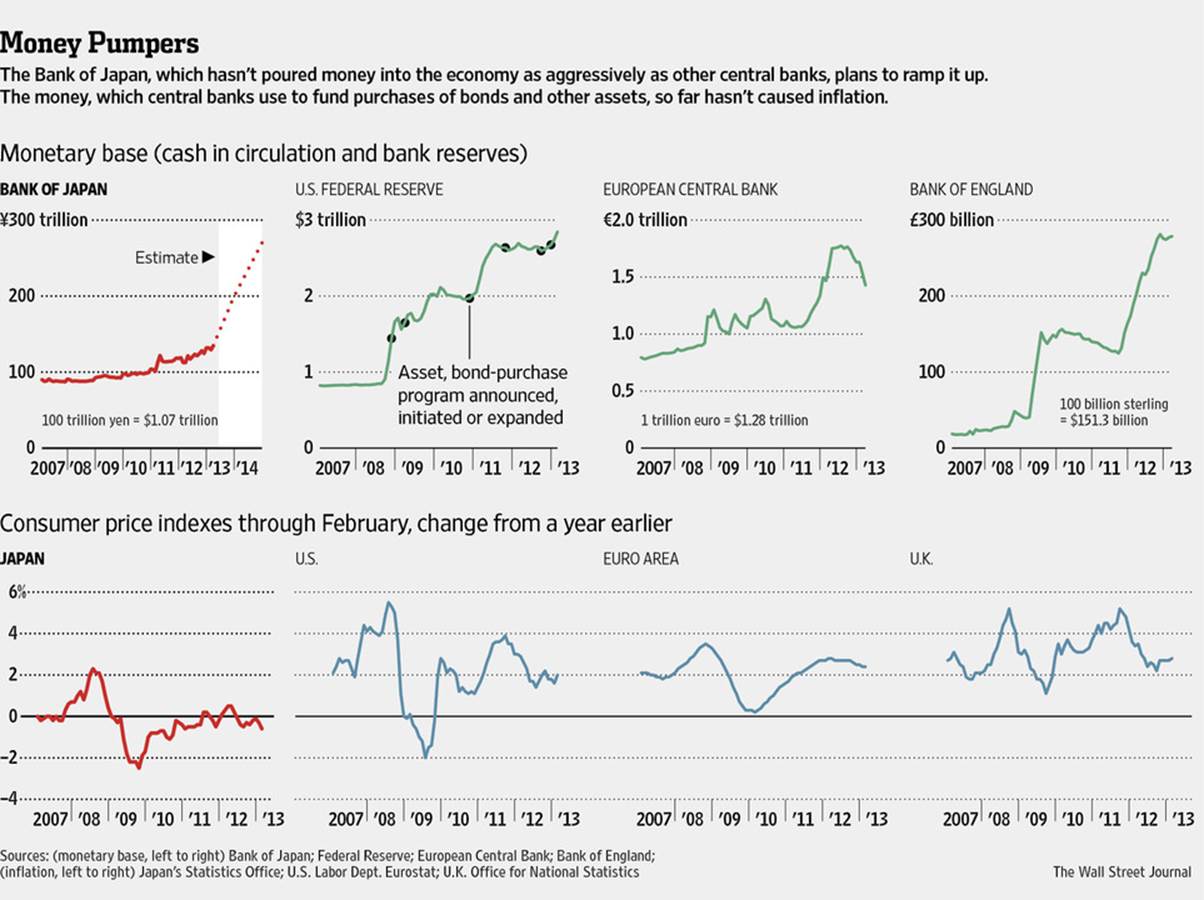
Money Spigot Opens Wider |
| Bloomberg Economics: Free 2 Month Trial Posted: 10 Apr 2013 11:30 AM PDT |
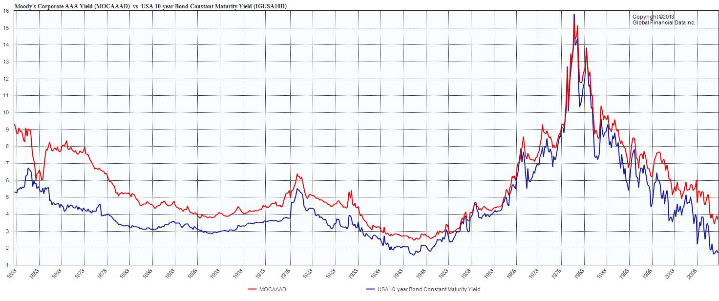
| Corporate AAA Yields vs 10 Year, 1857 – Present Posted: 10 Apr 2013 09:15 AM PDT Moody's Corporate AAA bond yields vs US 10yr Constant Maturity Yield to 1857
There is a tendency to look at the S&P500 Dividend Yields vs US 10 year, but in many ways, that is a less than ideal comparison. Corporate Bonds are more of an apple to apple comparison. Note that there is an almost 200 bps spread over the US 10yr — nearly double the dividend yield of the S&P500. We keep talking about how the "Great Rotation" into equities from bonds has not yet happened, but folks looking for yield may wish to pay more attention to AAA rated corporates. |
| Posted: 10 Apr 2013 07:00 AM PDT My morning reads:
What are you reading?
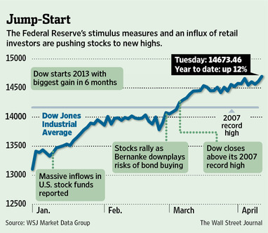
Dow Hits Record Amid ‘Absence of Attractive Alternatives’ to Equities |
| Why Canada Avoids Banking Crises Posted: 10 Apr 2013 04:23 AM PDT I am intrigued by the issue of how our own cognitive foibles impacts our decision making processes as investors. Our behaviors have evolved for other reasons (primarily survival); Regular readers know I am especially interested in how our wetware fails us when applied to making risk decisions in capital markets. It is exceedingly difficult to avoid these kinds of biases and cognitive errors in your own behavior, which is why smart investors develop rule based decision-making to help overcome these issues. It is, however, a rather simple task to identify cognitive errors in other people. I find myself constantly playing pop cognitive therapist as I watch massive rationalizations occur. I see them deployed to explain why stocks are rallying, or why the economy hasn’t collapsed yet, or why a fit of under reported inflation will soon lead to $7000 gold (ignore the falling prices for now). Probably the greatest example of bias is seen as some try to explain why the financial crisis occurred. Post bailout, the flailing, cognitive dissonance has been astounding. It is the underlying cause of the Big Lie. I was reminded of this while reading a Real Time Economics post on Why Canada Can Avoid Banking Crises and U.S. Can't. It discusses a new paper (and forthcoming book) by Charles Calomaris and Stephen Haber. The thesis is that Canada has a French legal history, which created a “highly-centralized federal government which controlled economic policy making and had built-in buffers for banker interests against populist forces” as the primary reason for its stability in banking. Calomaris is an economics professor at Columbia University. My experience with him is he’s a really nice, really smart guy. At a conference somewhere in the Caribbean (I think Cayman Island), we had dinner with the wives after our respective presentations. I am often interested in what his thinking is about economic topics. But it is his other role, as Co-Chair of AEI’s Financial Deregulation Project with Peter Wallison that raises questions in my mind. Back to Canada: The legal backdrop is a fascinating concept, one I want to explore further. But I cannot help but wonder if this line of thinking came about to avoid the obvious issues in the US, namely, the crisis was driven in large part by the radical deregulation. In Canada for example, there are other factors beyond the French legal history worthy of discussion. Note that in Canada, bankers cannot lobby regulators. Unlike the US, their Supreme Court does not think corporations are people. In Canada, money is not speech. There are explicit limitations on Corporate political donations. And where as we have a revolving door between government service and the private sector, the restrictions are much greater in Canada. All of this adds up to a much more intensely regulated banking system than in the America. Which makes me wonder how this will get treated in their book. It also raises important questions regarding academic objectivity. If your starting premise is that the financial system needs to be deregulated, how objective can any of your subsequent academic research be? If you spend time co-chairing AEI’s financial deregulation project, how much of your thought process is in part a rationalization of your own role in creating the crisis? (I’ll let someone else look into the issue of academic research being funded by deep-pocketed ideological Think Tanks). If your starting premise is deeply, fundamentally flawed, what happens to the academic theories built on top of that foundation? By all means, we should be looking at all of the factors that drove the credit bubble and collapse. We just need to be especially aware of the framework our own biases create when we do so . . .
Previously: Source: |
| Can Risk Aversion Explain Stock Price Volatility? Posted: 10 Apr 2013 02:00 AM PDT Can Risk Aversion Explain Stock Price Volatility?
Why are the prices of stocks and other assets so volatile? Efficient capital markets theory implies that stock prices should be much less volatile than actually observed, reflecting an unrealistic assumption that investors are risk neutral. If instead investors are assumed to be risk averse, predicted volatility is higher. However, models that incorporate investor avoidance of risk can explain real-world stock price volatility only under levels of risk aversion that are unrealistically high. Thus, price volatility remains unexplained. ~~~ The global financial crisis forcefully reminded us of the important effects of financial markets on the real economy. But it also renewed our appreciation of how difficult it is to demonstrate these connections successfully. Economists have mathematically elegant models of financial markets with strong theoretical underpinnings. They also have models that connect successfully with the data. However, few, if any, models do both. In financial economics, this is a time of uncertainty and searching for new directions. This Economic Letter summarizes developments in one important area of this field: asset price volatility. It is easiest to summarize financial markets research by focusing on the stock market, although the analysis can be applied to other financial markets with little modification. The earliest line of financial economics research that connects directly with current work is on efficient capital markets, developed in the 1960s and 1970s (Fama 1970). The defining claim of efficient capital markets theory was that, if investors process information efficiently and price stocks rationally, then future returns cannot be forecast. That's because, if returns could reliably be forecast to be abnormally high in the future, investors would buy stocks now. That would cause stock prices to rise immediately, bringing future returns down to a normal level. The reverse would take place if returns could be forecast to be abnormally low. Empirical research appeared to confirm that financial market returns can't be forecast.
Unfortunately, formal models incorporating risk aversion produce the degree of volatility seen in the real world only with levels of risk aversion that seem implausibly high. Thus, taking investor risk aversion into account does not satisfactorily explain the volatility of stock price movements. To understand this better, a recap of financial economics theory is helpful. Early stock market gurus such as Benjamin Graham and David Dodd (1940) held that stocks should be traded based on the relationship between their prices and the discounted value of their expected future dividends. This present value model assumed that the discount rate could be held constant. At first glance, the efficient markets model appeared to conflict with this present value model. However, Samuelson (1965) showed that, far from being contradictory, the present value and efficient markets models were essentially equivalent. If stock prices equal expected future dividends discounted at a constant rate, returns in fact can't be forecast. Further, the assumption that stock prices equal expected future dividends independent of the volatility of dividends can be justified only if investor risk aversion is excluded. If investors are risk averse, stock prices will depend on how variable dividends are as well as on their expected levels. By ignoring this effect, market efficiency implicitly treats investors as being risk neutral. In the 1970s and 1980s, empirical evidence that raised questions about the efficient markets model began to surface. Shiller (1981) and others showed that, under the efficient markets model, stock prices should exhibit the same low volatility as dividends themselves. By "price volatility," I mean the overall variability of stock prices over time. It is important to distinguish between this definition and a frequently used alternative definition of volatility as the average variability of stock returns, consisting of dividends plus price changes. To see the difference between price volatility and return volatility, assume unrealistically that investors have information that allows them to predict future dividends into the indefinite future with perfect accuracy. Then the present value model implies that stock returns are equal to the constant discount rate and have zero volatility. At the same time though, stock prices will still go up and down as dividends change, which means they will be volatile. Shiller's conclusion was based on the fact that the stock price volatility implied by a given dividends model depends on how much information investors are assumed to have about future dividends. If investors cannot predict future dividend growth at all, they will price stocks at a constant multiple of current dividends. The volatility of stock prices relative to dividends will be zero. On the other hand, if investors have information about future dividends, then stock prices relative to dividends will vary over time. The more information about dividend growth investors have, the greater the average price variation. The extreme case assumes that investors can forecast all future dividends. Therefore, the price volatility associated with complete information is the highest level of volatility that can actually occur. In exercises known as variance bounds tests, Shiller and others found that observed price volatility appeared to exceed this maximum level, contradicting the efficient markets model. Risk aversion It is easy to see why the efficient markets model implies low price volatility. The rate of return on stock is defined as the dividend yield plus the rate of capital gain. This relation can be shown to imply that price volatility relative to current dividends is due entirely to the degree that future dividend growth and future returns can be forecast. If investors can forecast variations in dividend growth, they will price stocks at a high or low multiple of current dividends depending on whether dividend growth is expected to be high or low. In fact, dividend growth empirically is nearly impossible to forecast, implying that price volatility can be attributed to it only to a very minor extent. The efficient markets model implies that future returns can't be forecast. It follows that the efficient markets model combined with the empirical fact that dividend growth is nearly impossible to forecast implies low stock price volatility. Thus, the degree of stock price volatility seen empirically can only occur if we reject market efficiency and hold that future returns contain a large predictable component. In view of the association of market efficiency with risk neutrality, it follows that the market efficiency assumption of risk neutrality must be rejected to allow for risk aversion. Economists have a measure of risk aversion. Suppose an investor were offered the prospect of either doubling his wealth or halving it, depending on the outcome of a random event. The higher the probability of success, the more prone the investor would be to accept such a gamble. The investor's risk aversion can be defined to depend on the minimum probability of success that would induce him to accept the bet. The higher the minimum probability he demands, the higher his risk aversion. An investor with no risk aversion would accept the gamble if the probability of success exceeded one-third because the gain under success is double the loss under failure. But risk-averse investors would require a higher probability of success. An investor who requires a probability of 0.5 is defined as having risk aversion of one. Table 1 shows other probabilities. A reasonable guess for the average investor's minimum probability is around 0.67, implying a risk aversion of about 2. Table 1
In a theoretical model, Lansing and LeRoy (2011) computed the stock price volatility implied by different levels of risk aversion. Like Shiller, they found that, under risk neutrality, predicted maximum stock price volatility is much lower than what is actually seen in the market. They also found that the higher the level of risk aversion, the higher the maximum stock price volatility. To generate a price volatility level near that seen in the real world, the model needs an implausibly high level of risk aversion around 4 or 5, implying a probability of success around 0.94 in the gamble described above. Most investors would not need such a high probability of success to accept the risk. What's more, risk aversion must be even higher if the stock price volatility implied by formal models is to be reconciled with actually observed volatility. Maximum volatility in the models is based on the implausible presumption that investors can predict dividends with perfect accuracy into the indefinite future. If investor ability to predict future dividends is more limited, then predicted price volatility will be lower under a given degree of risk aversion. Accordingly, still-higher levels of risk aversion are required to account for real-world price volatility. To summarize, allowing for risk aversion can in principle generate stock price volatility similar to that seen in real-world financial markets. However, that assumes either that investors are implausibly risk averse or that they can predict dividends into the distant future, or both. Otherwise, price volatility surpasses levels that can be explained by fundamentals. It follows that assuming that investors have reasonable levels of risk aversion is not enough to explain why stock prices are so volatile. Conclusion The finance models summarized in this Letter are at odds with empirical data. Economists have been experimenting with innovative models that might help explain why asset prices are so volatile. Some have been looking at behavioral models that don't assume full rationality, but these have problems of their own. So far, these investigations have not led to convincing explanations. It is far from clear where we go from here. ~~~ Stephen F. LeRoy is a professor emeritus at the University of California, Santa Barbara, and a visiting scholar at the Federal Reserve Bank of San Francisco. References Fama, Eugene F. 1970. "Efficient Capital Markets: A Review of Theory and Empirical Work." Journal of Finance 25(3), pp. 383–417. Graham, Benjamin, and David Dodd. 1940. Security Analysis. New York: McGraw-Hill. Lansing, Kevin J., and Stephen F. LeRoy. 2011. "Risk Aversion, Investor Information, and Stock Price Volatility." FRB San Francisco Working Paper 2010-24. Samuelson, Paul A. 1965. "Proof that Properly Anticipated Prices Fluctuate Randomly." Industrial Management Review 6, pp. 41–50. Shiller, Robert J. 1981. "Do Stock Prices Move Too Much to be Justified by Subsequent Changes in Dividends?" American Economic Review 71(3), pp. 421–436 |
| You are subscribed to email updates from The Big Picture To stop receiving these emails, you may unsubscribe now. | Email delivery powered by Google |
| Google Inc., 20 West Kinzie, Chicago IL USA 60610 | |


0 comments:
Post a Comment